
Land Cover Change Analysis
Using historic air photos to interpret and assess land cover change in the Annapolis Valley from 1931 to 2012
This work was done as partial requirements of a Master of Science in Applied Geomatics, a joint program at Acadia University and the Centre of Geographic Sciences [COGS, NSCC]. The project was sponsored by Clean Annapolis River Project [CARP]. Funding was provided by Mitacs Accelerate , with contributions from Environment and Climate Change Canada, the Nova Scotia Department of Natural Resources and Renewables, the Canada Nature Fund and Clean Annapolis River Project.
Land Cover Mapping
Land cover maps are utilized in almost every industry: science and research, conservation, resource extraction, urban planning, agriculture, health services, and more. They are used for gathering all kinds of useful information about the landscape, such as:
- locating natural resources
- identifying environmental risks and hazards
- to determine the composition of an ecosystem
- to observe weather and seasonal patterns
- measure the frequency and severity of natural disasters
- to assess agricultural or forestry capacity and production
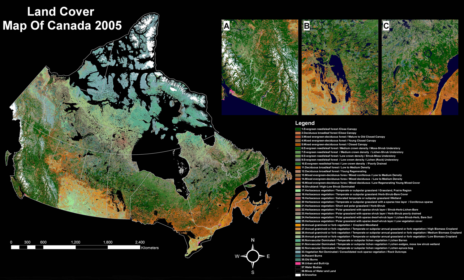
A Land Cover Map of Canada, produced by NRCAN, derived from MODIS (satellite) imagery.
This information can then be used to:
- develop sustainable land-use practices and policies
- understand the impacts of climate change and improve adaptation strategies
- monitor ecosystems to facilitate research and study
- inform emergency preparedness strategies and community resilience
When land cover is mapped over a significant period of time we can determine how and why the landscape is changing.
Understanding the history and change of a landscape improves our ability to plan, manage and mitigate impacts to our communities and ecosystems.
Land cover maps were originally produced by conducting field surveys, measuring and drawing up the features by hand, and creating a final printed map product. As you can imagine, this was time consuming, could result in wide margins of error, and was not created in a format easily accessed, edited or shared with others. Now, we can utilize mapping software known as Geographic Information Systems (GIS) and remotely sensed data to more efficiently produce dynamic digital land cover maps over large areas. These maps can be easily edited, updated, and shared online for improved accessibility and data sharing.
Remotely Sensed Data
"Remote sensing is the science of capturing information about the earth’s surface using reflected or emitted energy collected by sensors mounted on satellites, aircrafts or drones. " - Natural Resources Canada
Air photos are a type of remote sensing data, representing a specific moment in time. They are typically captured from an aircraft (helicopter, plane, drone), and comprise either film or digital photographs. The first air photo ever taken was in 1858 by hot air balloon over Paris - but unfortunately no longer exists. This image (right) is the oldest surviving air photo, taken by hot air balloon in 1860 over Boston.
It can often be the case that historic air photos are the only existing records available for a given place at a given time, consituting an incredibly valuable source of landscape information. Commercial aerial photography began in the 1920s and continues to this day, providing a detailed record of the earth's surface over time.
Considerations when using historic air photo data (film photographs)
- Images may be warped, torn or faded due to improper storage or poor film processing
- Colour, contrast and other visual interpreration qualities will vary due to the limitations of the technology of the time
- Most film photographs are not georeferenced (i.e. they contain no real-world locational information necessary for intergration with digital mapping software -- additional processing must be done to integrate this data with a GIS)
- Data may simply not exist for certain places at certain times.
- imagery was not always collected in a systematic manner
- physical copies may have been irreparably damaged or lost
Project Objective
The goal of this project was to map the land cover of the Annapolis Valley over time through air photo interpretation and determine what landscape changes may have impacted historic sand barrens. Said to have encompassed more than 200 km 2 in the past, the Nova Scotia Department of Lands and Forestry estimates that less than 3% of the original sand barrens remain. Urbanization, intensive agriculture and fire suppression resulting in dense reforestation are the most likely factors. Understanding the history of the Valley and evolution of the landscape will help us to develop targeted conservation strategies that benefit our communities while protecting a rare and unique Canadian ecosystem for generations to come.
Project Area
To begin this work, a project area had to be determined to find the right data and potential scope for assessment. The following elements were considered when identifying the project area:
- Regional Topography and Ecology
- The Extent and Composition of Sandy Soils
- Known Sand Barren Sites
- Availability and Overlap of Air Photo Data
- Processing Time Constraints
Navigate the maps by using the widgets in each corner and mouse to move around the frame.
1. Topography and Ecology
The Ecological Land Classification (ELC) guide, developed by the Nova Scotia Department of Natural Resources and Renewables, divides the province into ecological regions, districts and zones characterised by similar features, such as: climate, elevation, topography, bedrock formation, and vegetation.
ELC 2015 EcoDistricts of Nova Scotia
EcoDistrict 610: Annapolis Valley This mostly flat and warm valley, located between the North and South Mountain ranges, is known for its sandy glaciofluvial outwash plains that historically supported large heathlands -- a sand barren-like habitat. It is also the most heavily and intensely farmed district of Nova Scotia.
The original ECODISTRICT 610 data was modified for use as a Project Extent Boundary and trimmed down to within the historically known range of the Annapolis Valley sand barrens.
This boundary would be used to focus the analysis and clip datasets down in size to reduce processing and data storage requirements.
2. Extent & Composition of Soils
Provincial soil data was used to determine the location of primarily sandy soils throughout the Project Extent that have the potential to support sand barren ecosystems.
The 1:75,000 scale Detailed Soil Survey dataset (v3 ) was produced by the National Soil DataBase ( NSDB ) of Canada.
The field TSAND represents: Total Sand Content by Weight. The assessment focuses on TSAND values between 70-90% to identify areas most suitable for sand barren species.
3. Known Sand Barren Sites
There are a few known sand barren sites within the valley, identified by CARP and other ecosystem experts. The sites were used as guides for:
- land cover interpretation
- assess the factors most likely impacting current and historic sand barrens
- develop conservation recommendations and strategies
4. Air Photo Availability & Overlap
The earliest sets of Air Photo data (from 1931 and 1955) were acquired from the National Air Photo Library (NAPL) of Canada.
1931 & 1955 air photo details:
- scanned photos delivered in digital Tagged Image File Format (TIFF)
- only available in grayscale (black and white / singleband imagery)
- not georeferenced
- data not available across the entire Project Extent
Air Photo data from 1977, 1992 and 2012 were acquired from the Nova Scotia Geomatics Centre (NSGC) , also known as GeoNova.
1977 & 1992 air photo details:
- scanned photos delivered as TIFF files
- true colour imagery (3-Band)
- cover the majority of the Project Extent (specific data selected in 1992 for new assessment site, described later)
2012 air photo details
- available as 1:10 000 scale orthophotos
- already georeferenced
- true colour imagery (3-Band)
- covers the entire Project Extent
5. Processing Time Constraints
Because not all of the air photo data covered the entire Project Extent, a second site for assessment was established, named the Minor Area.
The Minor Area boundary was created by overlapping the limited air photo data with the known sand barren sites to establish the maximum overlap.
In order to create detailed land cover maps over frequent intervals of time, this smaller assessment area was necessary. Having two scales for analysis would also ensure that valuable historic information for the majority of the Annapolis Valley was preserved.
The project areas were now determined and two scales of assessment established:
Project Extent
Includes air photo data from 1931, 1977 and 2012. This encompasses 81 years of change in the Annapolis Valley at ~40 year intervals.
Minor Area
Includes air photo data from 1931, 1955, 1977, 1992 and 2012.
Detailed land cover mapping will show how a part of the Annapolis Valley has changed since 1931 at ~20 year intervals.
Explore the layers of data that were used to determine the project areas. Turn layers on and off with the Layer List and see the layer names and descriptions in the Legend (bottom-right widgets). Navigate the map by using your mouse to pan across the scene and the + and - widgets to zoom in and out (top-right).
Methodology
After establishing the project areas and selecting the appropriate data, the imagery was processed and integrated into the mapping software. Land cover was classified, mapped and measured to determine how change was occuring over time. Finally additional landscape data was incorporated to assess what changes were impacting sand barrens and suggest strategies for conservation and further assessment.
Air Photo Processing
The individual air photos were processed into orthomosaics for land cover mapping.
An orthomosaic is a large, detailed image made up of smaller orthophotos -- air photos that have been corrected for any scene distortions and terrain relief to create a top-down view of an area with uniform scale throughout.
Orthomosaicking was done with Agisoft Metashape Professional software involving the following steps:
Checking images for obstructions, clarity, and markings.
- All of the air photos were resampled and resized where necessary to create a uniform set of a manageable size. Large files can slow down processing and interpretation.
- Individual images are checked for visual quality and markings that can confuse the software processing.
E.g. Air photo from 1931, pictured (right)
- Shadows cast by objects or clouds
- Clear surface detail for interpreting land cover
- Watermarks and fiducial marks, typical of film photos
- Fiducial marks, watermarks and borders were manually masked out so that only ground features are processed by the software during alignment -- matching features between overlapping images and stitching them together.
Masking out markings from scanned photographs. No mask (a), and with mask (b).
4. The photos are then georeferenced, giving the scene real-world location information. - Ground Control Points were collected from the mapping software then imported and matched to the ground features in each air photo. - Newer cameras have location information built in to the sensors that speed up this process, but this remains a manual process with historic air photos. - Georeferencing is a necessary step to integrate the imagery with the mapping software.
5. The software completes the final steps of merging all of the photo details and geographic information together to produce an orthomosaic that can be imported to the mapping software for land cover mapping.
Land Cover Mapping
The land cover mapping was done in Esri's ArcGIS Pro .
The first step was to determine a system of classifying the land cover to be mapped. Classification often depends on:
- the amount of surface detail that can be identified from the image
- the type of change/phenomena being assessed
- the level of distinction required between land cover types
- other available data used
Two land classification datasets ( Cycle 1 and Cycle 3 ) produced by the Department of Natural Resources and Renewables' Forestry Division were used as the baseline for mapping land cover in 1992 and 2012, matching the photo year used for interpretation of the data. The land cover is divided into over 30 categories, many of which differentiate between types and compositions of tree stands. This level of classification was not necessary for this assessment, so the following schema was created to include and merge the Forestry categories into 6 distinct classes.
6 class land cover classifcation scheme with subclasses (e.g. Orchards) where possible.
Orchards found in 1931 imagery.
Agricultural areas are relatively easy to make out. Fields are typically rectangular with distinct edges and patterns from planting and harvesting can be seen from above. A subclass of Agriculture is Orchards. This crop type is also easy to differentiate from other ground features and are a staple crop of the Valley.
The Forest class represents areas of dense forest cover.
Wetland includes dry and wet bogs, treed bogs and any wet areas not included in the Water class, which represents open water bodies such as: lakes, ponds, and rivers.
The Urban class includes any buildings and industrial spaces. Subclasses include: Quarries and Roads.
The final Sparse Vegetation class is the best representation of what could be heathlands or sand barrens. It is made up of areas with low-lying, brush-like vegetation.
Results
With all of the mosaics completed, and land cover delineated, the classified areas can be calculated to observe land use during each period and landscape change over time.
Project Extent
The large mosaics, covering a majority of the Project Extent, from 1931, 1977 and 2012 show the general trends of change over time across the Valley.
1931
The 1931 orthomosaic has a ground resolution of 0.50 cm/pix.
The data covers roughly 42,354.94 hectares of the total. (Project Extent: 60,176.70 hectares)
Explore the imagery yourself by using the widgets to zoom in (+), out (-) and use your mouse to pan across the scene.
Orchards can be seen throughout the Valley.
An experimental Deep Learning Model was used to determine the coverage of orchards across the 1931 orthomosaic and accurately located at least 4,740.06 hectares. It is likely they made up a little more than 11% of the agricultural landscape at this time.
1931 to 1977
Use the swipe bar to observe the changes from 1931 to 1977. 1931 (left, grayscale) and 1977 (right, colour).
1977
The 1977 orthomosaic has a ground resolution of 0.37 cm/pix and covers 47,165.90 hectares.
The colour variation across the scene is due to photographs taken on different days and time of year. Most were captured in June and July however a few images were captured in October when land cover may appear different as foliage falls in the autumn and fields are harvested at the end of the growing season.
This was a period of considerable urban development.
You can see the construction of a new highway (Highway 101) cutting through agricultural fields and forests and many new smaller roads indicating new residential areas.
There are much fewer orchards and those that remain are more densely concentrated.
1977 to 2012
Use the swipe bar to observe the changes from 1977 to 2012. 1977 (left) and 2012 (right,).
2012
The 2012 orthomosaic has a ground resolution of 0.25 cm/pix and covers 56,566.37 hectares.
At this point in time, very few orchards remain although there is still a lot of land being used for other agriculture.
Areas that were cleared for development in 1977 are now complete and the spaces in between are filled by trees.
Forest cover in general has increased across the Valley and very few sparsely vegetated landscapes remain. This is more acutely noticeable when comparing the 1931 to the 2012 imagery.
1931 - 2012
Use the swipe bar to observe the changes from 1931 to 2012. 1931 (left, grayscale) and 2012 (right, colour).
1931 - 1977 - 2012
Explore all of the Project extent data from Orthomosaics to sandy soil data to see how the Valley has changed over 81 years!
Turn layers on and off with the Layer List, and see the layer names and descriptions in the Legend (bottom-right widgets). Navigate the map by using your mouse to pan across the scene and the + and - widgets to zoom in and out (top-right).
Minor Area
The Minor Area focuses on ~7,000 hectares of the Valley including the encompassing the communities of Aylesford, Greenwood and Kingston. Chosen mainly because of known existing sand barren sites in the area, but also to maximize the amount of air photo overlap. Interpretation and delineation of the land cover resulted in 5 fully classified maps used to calculate the landscape change over 81 years in roughly 20 year increments.
Although a portion of the 1931 and 1992 imagery does not cover the scene resulting in some No Data values (no classified land cover), the general trends observed throughout the Project Extent, can also be observed within the Minor Area.
When the No Data values are excluded, and the land cover results seen side by side (graphed below), the trends of urbanization and reforestation are clear. While dedicated agricultural space has somewhat decreased over time, the greatest land cover loss has been of the sparse vegetation class.
When viewed by photo year, the rate and extent of change is better understood.
1931
Mosaic ground resolution: 0.479 cm/pix Use the swipe bar on the map (left) to see how the land classification was completed using the air photos from 1931.
No Data values are for areas where no air photo data exists and where land cover could not be determined.
The 1931 landscape was predominantly dedicated to agriculture, making up 43% of the total classified area (No Data values excluded). Orchards, an established part of the Valley at that time, accounted for 20% of that agricultural space.
The second most dominant land cover type was sparsely vegetated areas, making up 22% of the area. Considering the portion of Minor Area in 1931 for which no air photo data exists and land cover could not be determined, it is likely that there was even greater coverage of both agricultural and sparsely vegetated spaces at this time.
Soils with significant (≥70%) and greatest (≥85%) total sand content were mostly utilized for agriculture but were also clearly characteristic of those sparsely vegetated areas.
1955
Mosaic ground resolution: 0.699 cm/pix Use the swipe bar on the map (left) to see how the land classification was completed using the air photos from 1955.
By 1955, significant urban development had taken place. Urban cover increased by 11%, mostly replacing sparse vegetation. A significant portion of this change is attributed to the development of the Canadian Forces Base in Greenwood.
There is little change to open water and wetland areas but forest cover increases by 5%, notably in areas of greatest sand content.
As urban spaces increase, it is likely fire suppression efforts also increased to protect these newly developed spaces. If fires were helping to keep forests at bay and stimulate the sparse vegetation species, it is possible a strategy of prescribed burning could reinvigorate those landscapes.
1977
Mosaic ground resolution: 0.372 cm/pix Use the swipe bar on the map (left) to see how the land classification was completed using the air photos from 1977.
Roughly twenty years later, in 1977, forest cover has continued to gradually increase and sparse vegetation continues to decrease.
There was another considerable 13% increase in urban areas -- this time reflecting a nearly equal, 11% loss of agricultural land. Urbanization was also occurring in areas of high sand content -- now representing the majority land cover type in all soils with sand content greater than or equal to 70%.
If areas of predominantly sandy soils are being developed into permanent urban spaces, this presents a real challenge for sand barren restoration efforts. A possible solution would be to redesign community green spaces to include more sand barren species and encourage home owners to plant these species in their own gardens.
1992
Mosaic ground resolution: 0.386 cm/pix Use the swipe bar on the map (left) to see how the land classification was completed using the air photos from 1992.
Similar trends observed in 1977 were observed in 1992, however the 6.5% increase in urban areas appears to have more significantly impacted sparsely vegetated areas than agricultural lands over this period.
Very little sparse vegetation remained by 1992, having lost 85% of the coverage represented in 1931. The loss is likely greater considering the gaps in the 1931 dataset bringing the totals nearer the estimations of previous studies that calculated a 97% loss of historic heathlands throughout the Annapolis Valley.
2012
Mosaic ground resolution: 0.250 cm/pix Use the swipe bar on the map (left) to see how the land classification was completed using the air photos from 2012.
Lands dedicated to agriculture stabilized by 1992 at 20% coverage with only a 0.3% increase in 2012.
Similarly, urban areas, which had been rapidly expanding until 1992 appeared to have plateaued, decreasing by 2% in 2012.
Forest cover continued to steadily increase over time, gaining another 2.6% between 1992 and 2012 marking a nearly 12% increase over 57 years (from 1955 to 2012).
The decreasing rates of change in 2012 show that land use has become more concentrated. If the land is not being used for agriculture of urban development, it is left to regrow into the dominant plant species. If those dominant species are also invasive, and are not monitored or managed, native and rare species -- such as those found in sand barrens could disappear from the Valley completely.
1931 to 2012
Zoom in, and compare all of the orthomosaics yourself to see how the Minor Area has changed over 81 years. Highlighted in orange are all of the dominant orchards from 1931. Use this layer to see what orchards survived until 2012.
Use the + and - widgets to zoom in and out of the map (top-right widget). The orthomosaics are only visible at close scale, zoom in to see imagery. Use the Layer List (bottom-right) to turn layers on and off and focus on specific mosaics/ periods in time.
Reforestation and urbanization appear to be the primary factors, each occupying roughly 11% more of the significantly sandy soils (≥70%) in 2012 than in 1955. In areas of greatest sand content (≥ 85%) urbanization increased by 21.5% in that 57 year period whereas forests only increased by roughly 9%. This indicates that the soils most likely to support sand barren ecosystems have been developed or are privately owned.
Involving communities and local stakeholders in sand barren restoration will be key to the success of these efforts.
The final aim of this project was to present the data in a dynamic format that would allow viewers to engage with the results and better understand how and why change was occuring. While the maps presented so far give a good sense of those trends, the beauty of a GIS and online sharing platform, is that data can be visualized in many different ways.
For this reason, a dashboard is used to compile the results in a single map frame and more easily intract with the various layers. In particular, the known sand barren sites.
Dashboard
ArcGIS Dashboards
This project provides important historical information about the landscape of the Annapolis Valley and the significant changes that have occured since the 1930s. It has demonstrated the value of air photo data for evaluating and mapping land cover. There is still more we can learn from the imagery and by utilising the maps for other analysis.
Future Projects
- Land cover classification could be completed to the full extent of the Project where data exists to see if the trends observed in the Minor Area are reflected across the Valley.
- Incorporate additional air photo data to observe change over smaller increments.
- Air photo data of the valley exist for the 1940s, 60s, 80s, and early 2000s. These could be incorporated to examine the rates of change over time to possibly isolate factors or specific events.
- Incorporating other sand barren data. As understanding and study of sand barrens increases, related data or parameters could be used to better interpret the land change results.
- Use an ecologically determined threshold of total sand by weight.
- Determine if historic fire records exist that can be mapped to better examine the relationship of fire suppression and sand barren loss.
- Locate and map sand barren-related species to determine if general reforestation is detrimental to the ecosystem or if specific species (e.g. Scots Pine, Pinus sylvestris) are inhibiting their growth.
- Incorporate property boundary information to determine the stakeholders of historic heathlands. Because much of the valley is privately-owned, stakeholder engagement and involvement will be key to successfully protecting sand barrens in the long-term.
The completion of this project would not have been possible without the contributions of many people. Foremost thanks to my academic advisor David Colville (COGS, NSCC), who inspired my continued education and career in geospatial science. Your guidance and encouragement kept this project going through the many unexpected challenges, and I will consider your counsel in all my future work! A warm thanks to my academic advisor Dr. Ian Spooner (Acadia), who was always willing to advise, support, and engage in my process and learning despite his busy schedule. Final, and special thanks to CARP members, Katie McLean, Brittni Scott and Gillian Kerr, and the members of the Sand Barrens Committee for their enthusiasm and support. You made it all possible.
Thank you!


